Fisher's iris data is very widely used. It was published in an article by Anderson in 1935. In 1936 Fisher, the well-known English statistician used it in an article proposing linear discriminant analysis, or Fisher's linear discriminant analysis. This method is now a central one, when it comes to classifying data, and provides the same result as that provided by simple learning machines such as the perceptron. The data consists of 3 varieties of iris flower, each providing 50 samples. There are measurements on 4 variables, petal and sepal length and breadth. The data matrix is therefore one of dimensions 150 x 4.
The Fisher iris data can be handled quite adequately by Fisher's and other well-tried and well-practised methods. For small dimensional data such as Fisher's (dimension = 4, for the samples) many methods are available. But with higher dimension, we have what Bellman referred to as "the curse of dimensionality": what worked fine in small-dimensional spaces fails completely due to scalability problems in higher-dimensional spaces.
To simulate a higher-dimensional problem, and to remain with the familiar properties of the Fisher iris data, we generated a recoded version of the Fisher data. For each of the 150 samples, we took the 4 given measurements, and made a much larger vector from them, - as it happens a 147-valued binary (0 or 1) vector. This was done simply by taking each 0.1 interval of each variable as defining a new variable. You can check the veracity of this data recoding by looking at a principal components analysis of the original data, i.e. the optimal 2-dimensional projection of the 4-dimensional space; and a correspondence analysis of the recoded data, i.e. an optimal 2-dimensional projection of the 147-dimensional space.
While traditional methods have increased computational difficulty in dealing with higher-dimensional spaces, this is just what a wavelet transform approach thrives on.
Let's look at the analysis of the 150 x 147 Fisher data. First we permute rows and columns though. Why? - because later will will look for contiguously-formed clusters, and therefore we need a canonical ordering of some sort to make this possible. There are lots of methods which give relatively similar permuted results. The one used by us was to take a principal components analysis of the 150 x 147 data and use the order of the pricipal component projections. (Why didn't we use the correspondence analysis result, since this is more appropriate for the boolean data used as input? For a minor technical reason: the correspondence analysis deleted columns among the 147 which had zero totals, thus not providing a convenient 147-valued set of ranks for us to work on). The reordered data used is shown as follows.

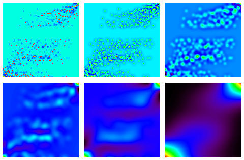
The à trous wavelet transform with 5 resolution scales and a residual gives the following. When added, these give a smoothed (with the scaling function used by the à trous method) version of the input data.

Supposing now that we are dealing with signal in the form of clusters or clumps of samples/measurements, and further that this nice view of our data is sullied by spurious information in the form of (low-count) Poisson noise, we filter our data.
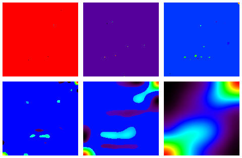
The multiscale 3-sigma detections based on these assumptions are shown in the following sequence of images.

The 5th scale, here, looks the most informative in terms of our set of 150 samples, divided as we know into three classes each of 150. The samples are represented on the horizontal axis. Taking the positive parts of this image, and taking everything above 0 as equal to 1 gives the following.

Reading off the sample numbers from the horizontal axis gave a credible result. For the first Fisher cluster, corresponding to the upper right cluster, one substitution error was found. The other Fisher clusters are a little less resolved, but - cf. the correspondence analysis output of the 150 x 147 data accessible above - are quite consistent with the input.
In dealing with the curse of dimensionality, therefore, we have a method which is fast and provides a good-quality result. And most of all, it thrives on high dimensionality problems.
Commands used
For the wavelet transform
mr_transform -x in.fits out
which produes out_scale_1.fits etc.
Next for the support image shown above, we have first run mr_abaque -d
to produce the file Abaque.fits.
Now we run
mr_support -I in.fits out
which produces the multiscale (weighted) support images in out.mr
which are then extracted using
mr_extract -x out out,
which produces out_scale_1.fits etc.
To probe further
For high-dimensional array reordering, see e.g. "Computational methods for intelligent information access", M.W. Berry, S.T. Dumais and T.A. Letsche, University of Tennessee, 38 pp., 1997, and other papers.
For some matrix reordering (or, better, permuting methods) see e.g. F Murtagh, Multidimensional Clustering Algorithms, Physica-Verlag, 1985.
For the filtering methodology used, see F Murtagh and J-L Starck, "Pattern clustering based on noise modeling in wavelet space", Pattern Recognition, 1998, in press.
Image and Data Analysis: The Multiscale Approach, J-L Starck, F Murtagh and A Bijaoui, Cambridge University Press, 1998.