MR/1 Edge Detection

• ERS SAR and SeaWiFS images of the Gulf of Oman containing several spiral features.

  Background description.

  Original SAR image.

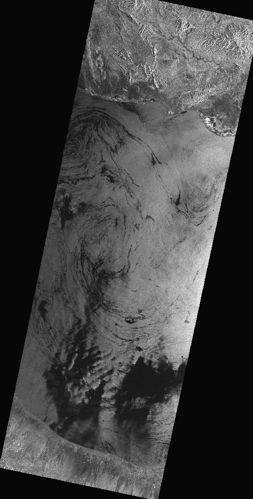
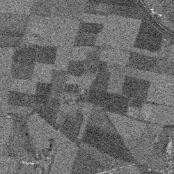
  SAR image superimposed on edge image.

  Commands used here:

  mr_at_edge -n 6 Qubsar.fits xxx
  mr_extract -s 4 xxx.mr zero1
  mr_extract -s 5 xxx.mr zero2
  mr_extract -s 3 xxx.mr zero3
  mr_extract -s 2 xxx.mr zero4
  mr_extract -s 1 xxx.mr zero5
  Then in IDL:
  IDL> a  = readfits('Qubsar.fits')
  IDL> s1 = readfits('zero5.fits')
  IDL> s2 = readfits('zero4.fits')
  IDL> s3 = readfits('zero3.fits')
  IDL> s4 = readfits('zero1.fits')
  IDL> s5 = readfits('zero2.fits')
  IDL> write_jpeg,'Qubsar-lev4.jpg',bytscl(hist_equal(100*s3+20*s2+a))
  

  Original SeaWiFS image.

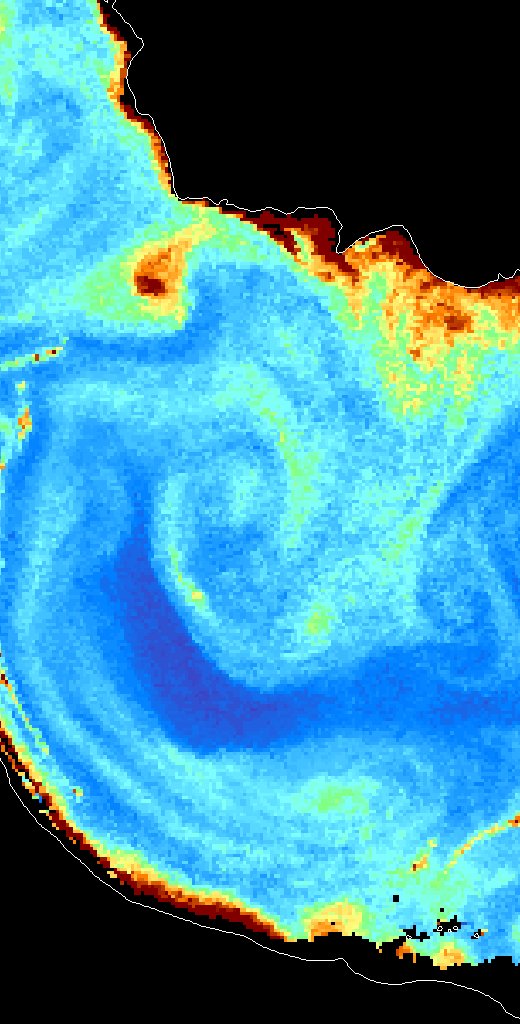
  Original SeaWiFS image superimposed on edge image.

  Commands used:

  mr_at_edge -n 8 Qubsw.fits Qubsw
  mr_extract -s 5 Qubsw.mr zero5
  Etc. for other bands.
  In IDL:
  a = readfits('Qubsw.fits')
  a5 = readfits('zero5.fits')
  write_jpeg,'Qubsw-lev5.jpg',bytscl(hist_equal(a5+0.0005*a))
  

  Level 5 of a multiscale median transform.

  Commands used:

  mr_transform -t 4 -x -n 7 Qubsw.fits wxy
  Above can take quite a while (e.g. 15 minutes on a Sparc 10 machine for 
  a 500x1000 image).  Scale or band 5 is shown above.
  

• A SAR agricultural image used in Chris Glasbey's Royal Statistical Society paper.

  Original image.

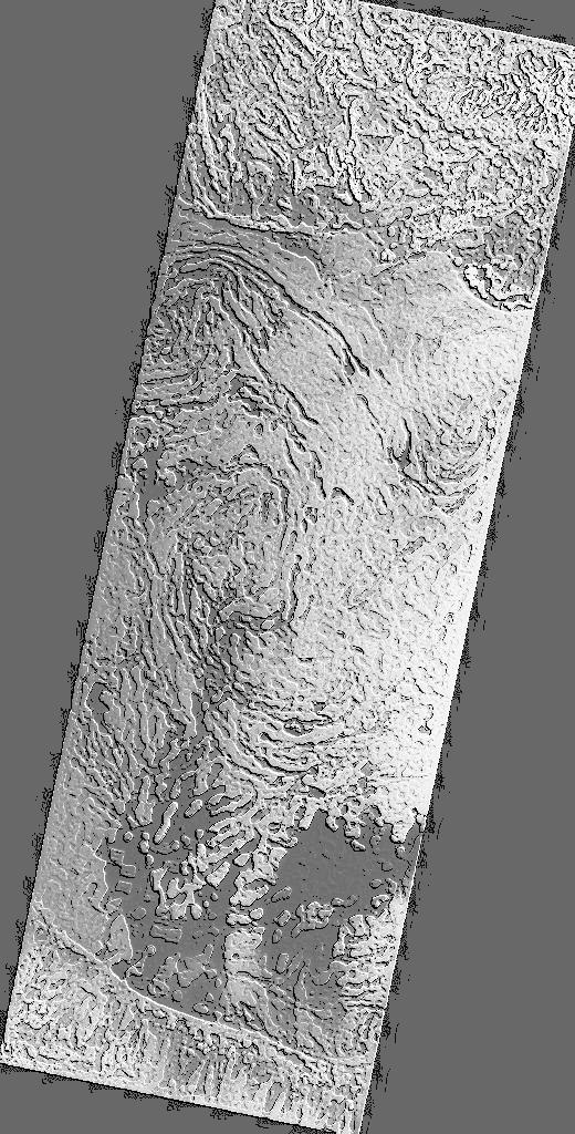
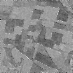
  Second derivative map (sar-proc5 below).

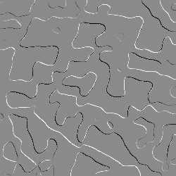
  Zero crossings superimposed on original image (sar-proc4 below).

  Commands used:

  mr_at_edge -n 6 sar.fits yyy 
  mr_extract -s 4 yyy.mr Zero4
  Etc. for -s 1 to 6
  
  In IDL
  a = readfits('sar.fits')
  zz4 = readfits('Zero4.fits')
  
  write_jpeg,'sar-proc4.jpg',bytscl(30*zz4+median(a^0.25,5))
  write_jpeg,'sar-proc5.jpg',bytscl(zz4<0.005)  (Slightly retouched in xv)
  

• Image used for processing - part of the image (identification removed).

  Scale 4 of second derivative map.

  Scale 5 of second derivative map.

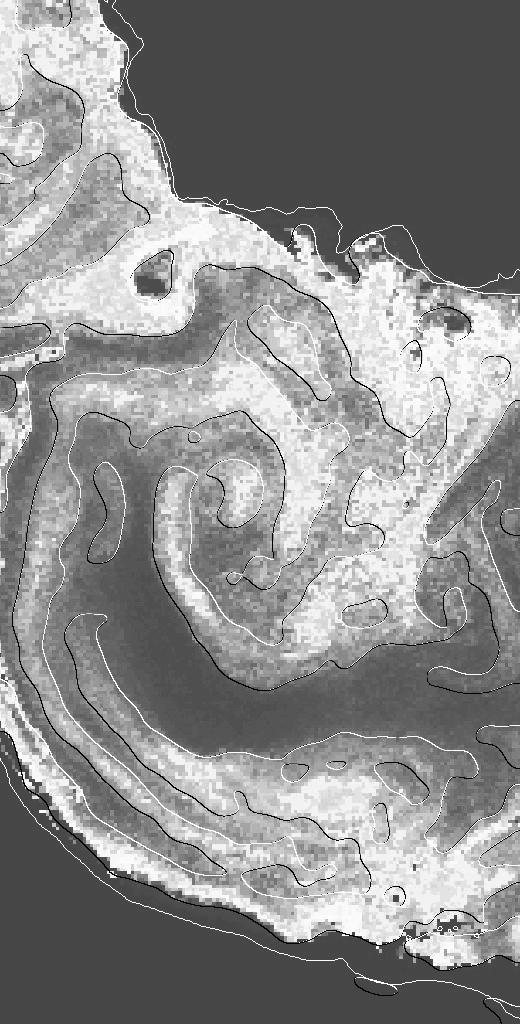
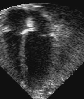
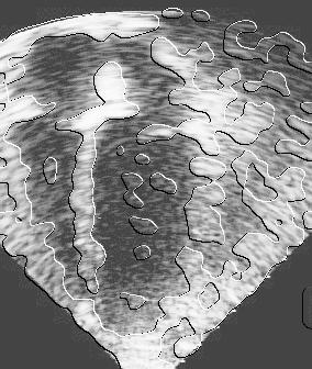
  mr_at_edge -n 5 asmi14cutout.fits asmi14cutout
  mr_extract -s 1 asmi14cutout.mr zero1
  mr_extract -s 2 asmi14cutout.mr zero2
  mr_extract -s 3 asmi14cutout.mr zero3
  mr_extract -s 4 asmi14cutout.mr zero4
  mr_extract -s 5 asmi14cutout.mr zero5
  
  In IDL:
  
  c = readfits('asmi14cutout.fits')
  s4 = readfits('zero.fits')
  s4_log = readfits('zero4_log.fits')   
  (Processed in the same way; data log transoformed.)
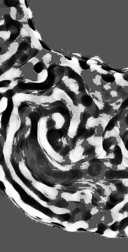
  write_jpeg,'heart_e1.jpg',bytscl(hist_equal(500.0*s4+c))
  write_jpeg,'heart_e2.jpg',bytscl(hist_equal(50000.0*s4_log+c))